My 31 MHz Phase interferometry telescope is ready. It uses 2 antennas (with a small amplifier), 2 coherent receivers,
a digitiser, a 130 m. long rs485 link to a normal windows XP computer at home.
The receivers are designed by H. Jenniskens ( Avisec ) and are direct conversion single sideband receivers
with a Weaver detector.
Both receivers use the same local oscillator (Si570) which is
controlled by an AVR microcomputer to change frequency.
The digitiser does sample both receiver signals every minute.
The first sample is from receiver A and the second sample is from receiver B.
A sample and hold circuitry is used to get the samples at exact the same time.
the next sample is again from receiver A and so on.....
It does about 32000 samples per second during 0.5 second.
So both channels get 8192 samples for one measurement.
The first real map
( i hope )
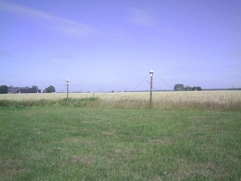
The two antennas. The poles are about 2 m. high.
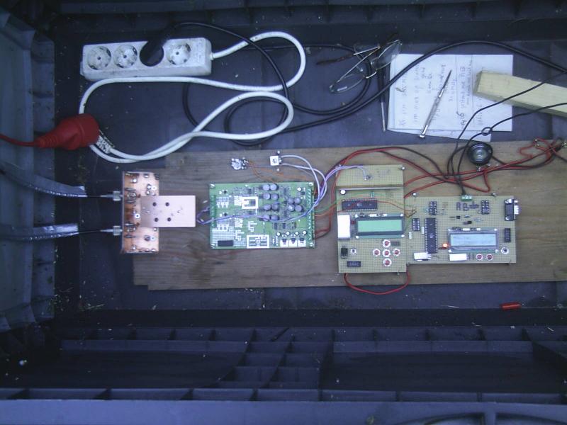
Above the receiver and the digitiser.
The copper unit at the left is the bandfilter for suppressing frequencies other than 31 MHz.
Right of the copper unit is the smd-circuit board on which are the 2 identical receivers.
More to the right is the circuit board of the AVR computer controlling the local oscillator
(si570) of the two receivers.
At the right is the circuit board which contains the digitiser and the rs485 convertor.
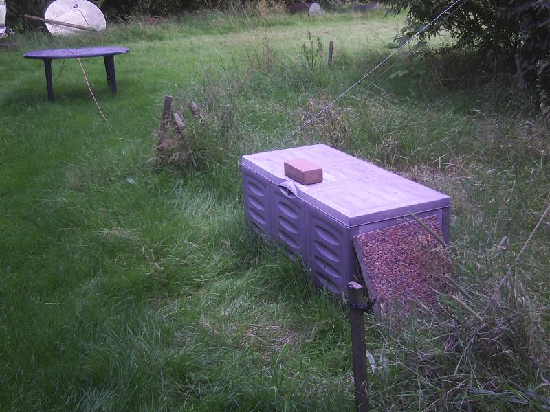
The receiver is hidden in a plastic box somewhere in the field between the 2 antennas.
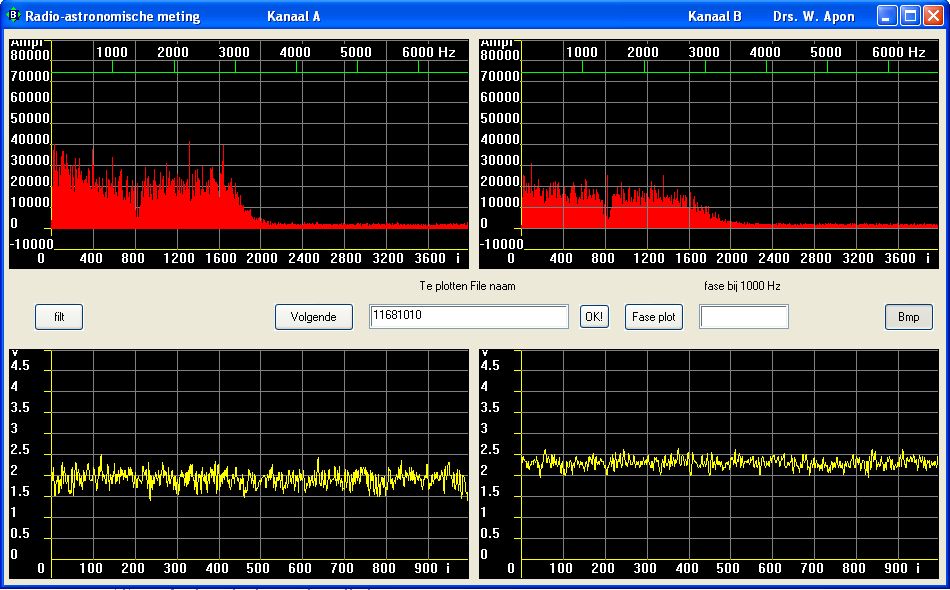
Upper left is the frequency distribution of the star-noise on channel A.
( The result of a Fast Fourier Transformation of 8192 samples)
Lower left is the received signal of channel A itself. (The first 1000 samples)
Upper right is the frequency disbribution on channel B.
Lower right is the received signal of channel B itself.
And now the core business:
How to calculate the crosscorrelation value of the two antenna signals:
You do every minute a measurement.
One measurement takes about 0.5 sec. In that time you get about 8000 samples from both antennas.
Now you start the crosscorrelation calculation.
What you do is: multiply the first number x(1) from the first antenna with the first number y(1) from
the second antenna.
Do this for every pair of numbers.
Sum all this products and devide it by the total number of numbers.
(x(1) * y(1) + x(2) * y(2) + .......... + x(n) * y(n) ) / n
So you get a number for every measurement.
This number is the crosscorrelation value.
Plot this numbers against the time of the measurement en you get a graph like below.
The white dots are this numbers.
Because this dots are jumping to wild, i calculate a running mean over some 20 numbers.
That is the red line in the graph below.
It looks very simple, but it is a magic trick.
This way of calculating omits the noise from the receivers but gains the noise coming from
the stars..... this is because the noise from the stars is the same ( coherent ) and the noise
from the receivers are different.....
So you throw away the receiver noice and amplify the noise from the stars!
Above a splendid measuring during the morning of 20-july-2010.
The Base: 102.58 m. West-East frequency: 31.0 MHz antennas: 2 times inverted V.
A perfect fit with CasiopeiaA simulation (Blue)
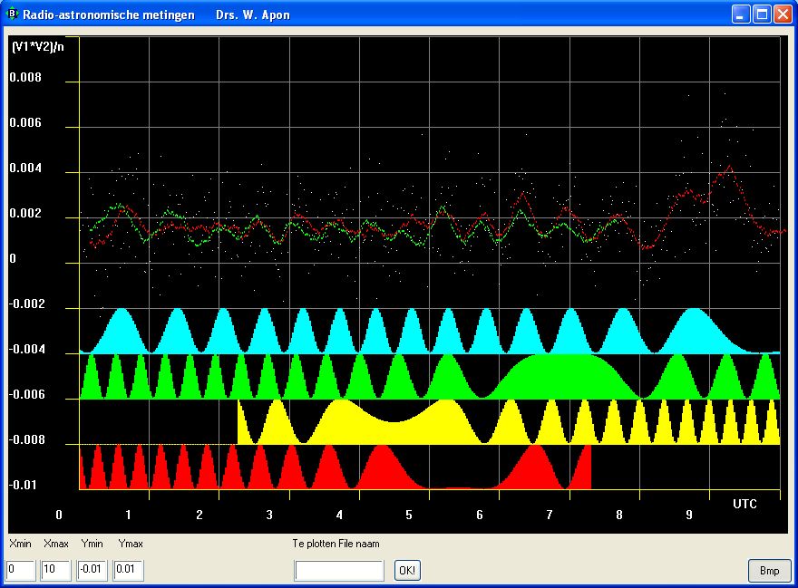
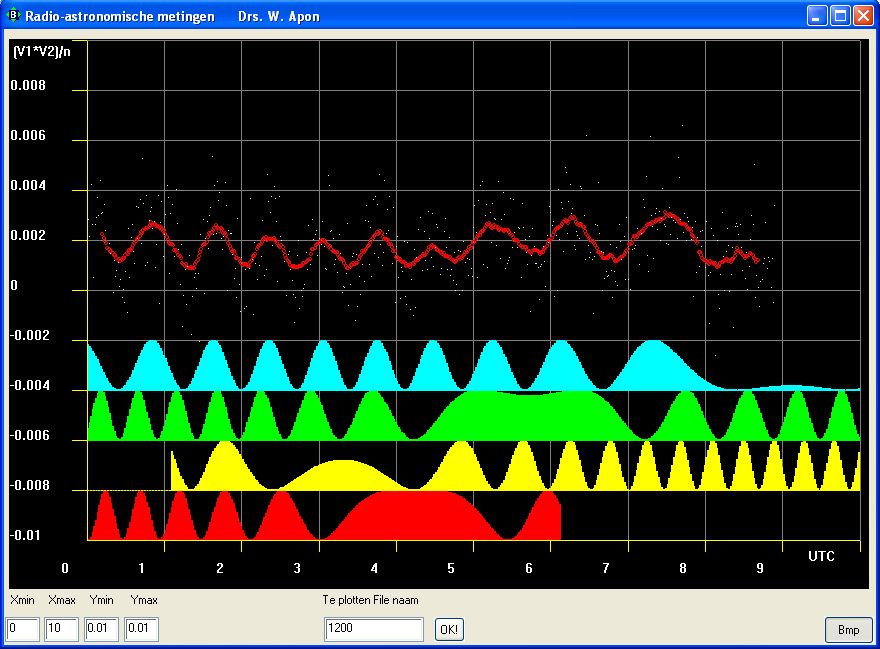
Two days measuring during the night.
The Base: 139.05 m. West-East frequency: 31.0 MHz antennas: 2 times inverted V.
below the 4 simulations:
upper : CassiopeiaA (Cyan)
middle: CygnusA (Green)
middle: TaurusA ( Yellow)
below : Top Milkyway (red)
The red curve is the first night and the green curve is the second night.
You can clearly see the daily 4 minutes difference between the two curves.
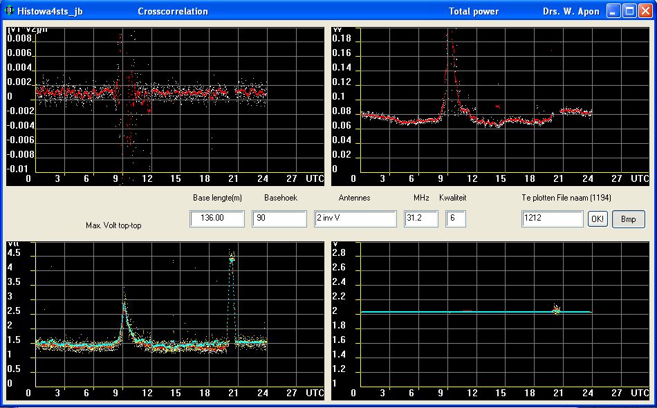
I got the sun burst at 1 august 2010 at 09:00 UTC.
Above you see the crosscorrelation, the total power and the maximum top-top voltage
of the received signal.
The second burst is a terrestrial noise signal.
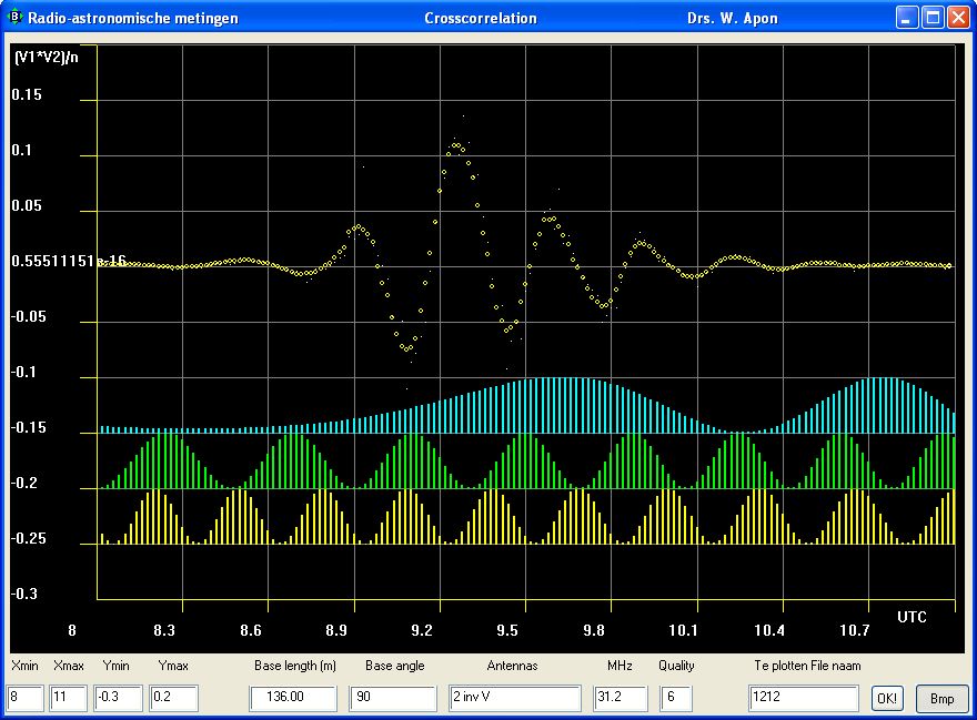
The crosscorrelation of the sun burst at more detail.
A splended graph.
When someone can tell me how many Jansky the burst was, i can calibrate my receivers!

The AstroRover.....
To be able to start a mapping program, i made my AstroRover.
I put the antenne on an old metal frame of a caravan, and so i
can move the antenna to any place i want in a few seconds.
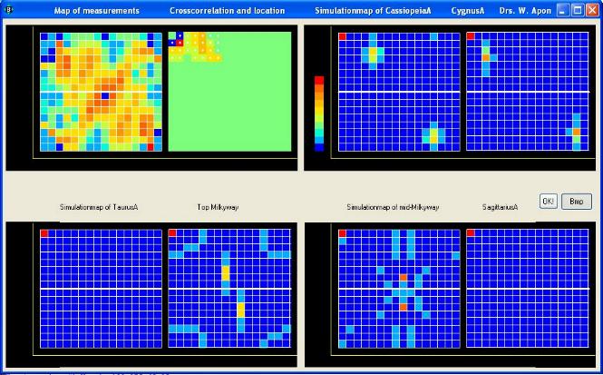
Unbelievable: it looks like a map of the sky. (Only the upper half of the pictures)
Upper left you see the map calculated by a 2d_fft of 24 measurements.
Time = 20:42 MST
See this as a picture of the sky of 0.0003 Megapixel.....
Right of this map you see a location map of the measurements.
A white dot is a measurement and the color of the pixel is the
crosscorrelationvalue of the measurement at this location.
The upperleft pixel is the location of the first antenna.
The second antenna has been placed on the other white dot positions.
Upper right you see a simulation at the same time of CassiopeiaA
and CygnusA
Below left is a simulation of TaurusA ( not visible at this time) and
The most high part of the radio-milkyway.
Below right is a simulation of The middle of the radio-milkyway and
SagittariusA ( not visible at this time)
If you take some distance from your screen you can see 4 sources:
(The orange parts.)
They seem to be, CygnusA and CassiopeiaA at the upperleft part of the map.
the Milkyway in the lower middle running to the upperright part.
I can make a map for every minute of the day,
but i have to say: most times the calculated maps do not resemble to the
simulations... so, is it a map or is it just par hasart ........or is there
a lot of disturbance of all kinds of factors like clouds, rain, etc.