Now working on:
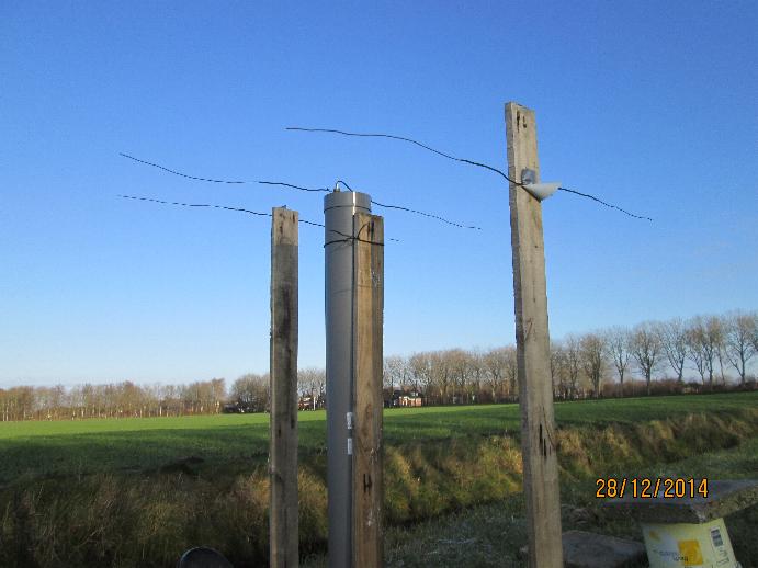
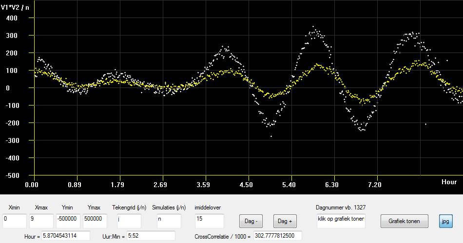
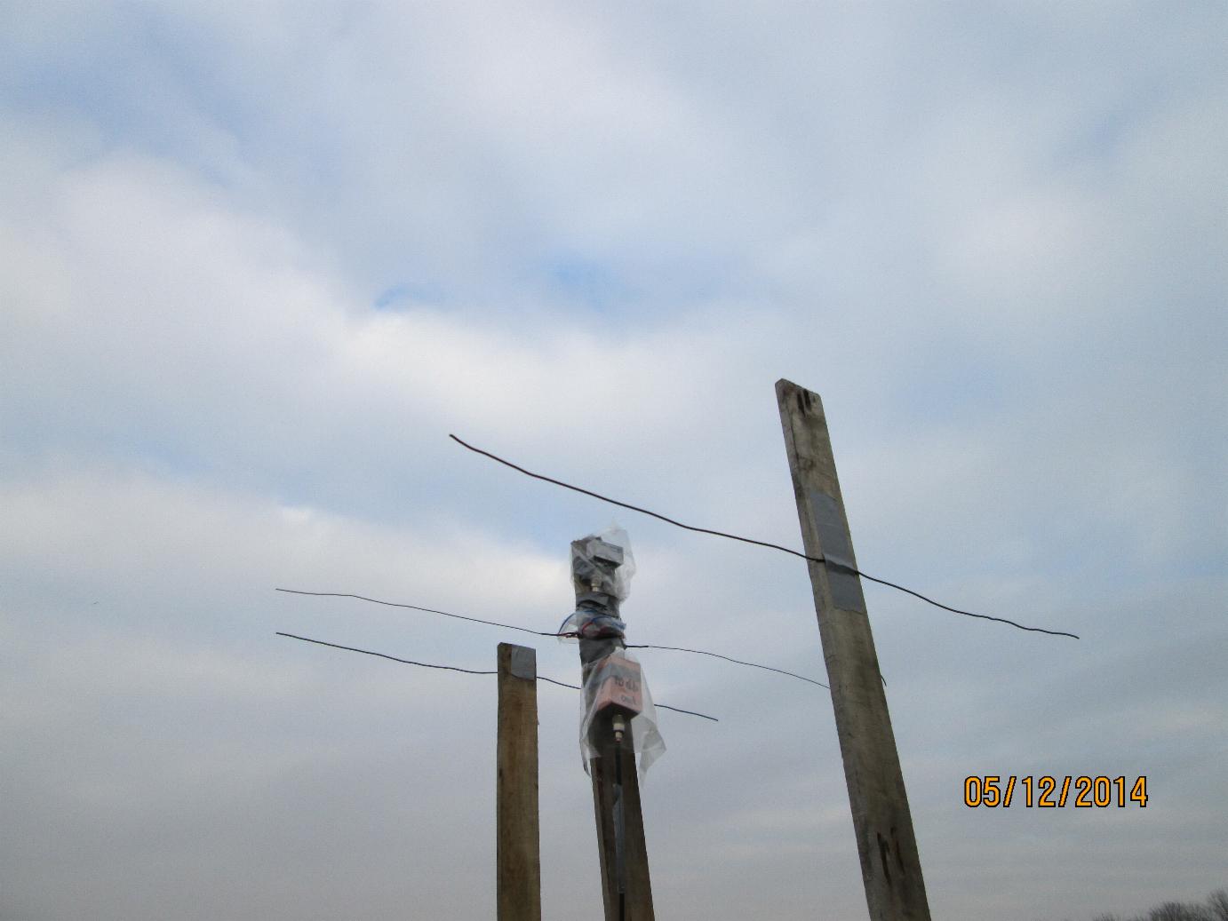
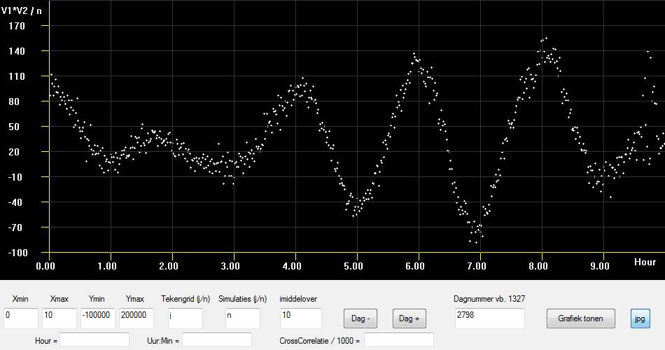
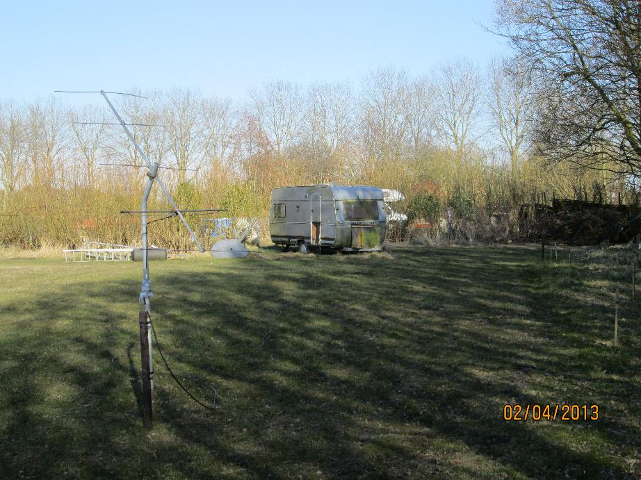
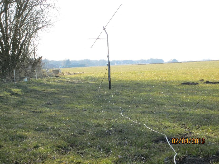
My SETI-station is ready and working.
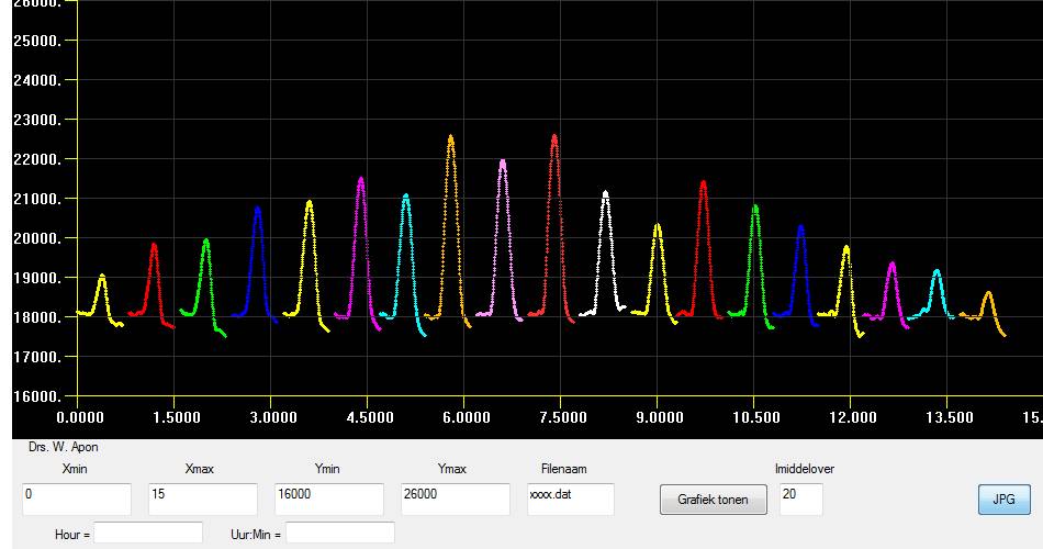
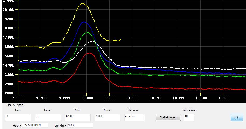
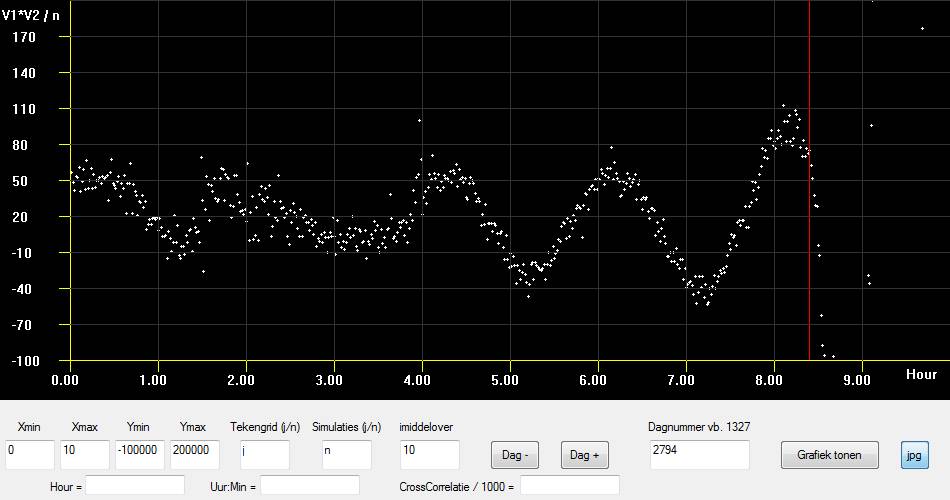
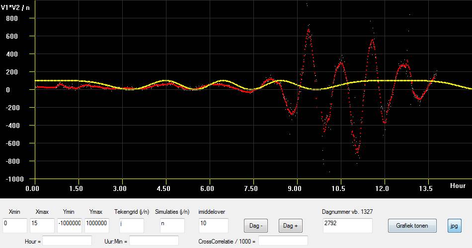
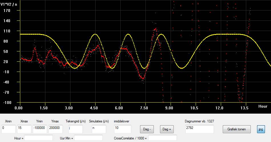
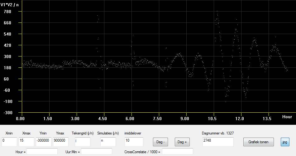
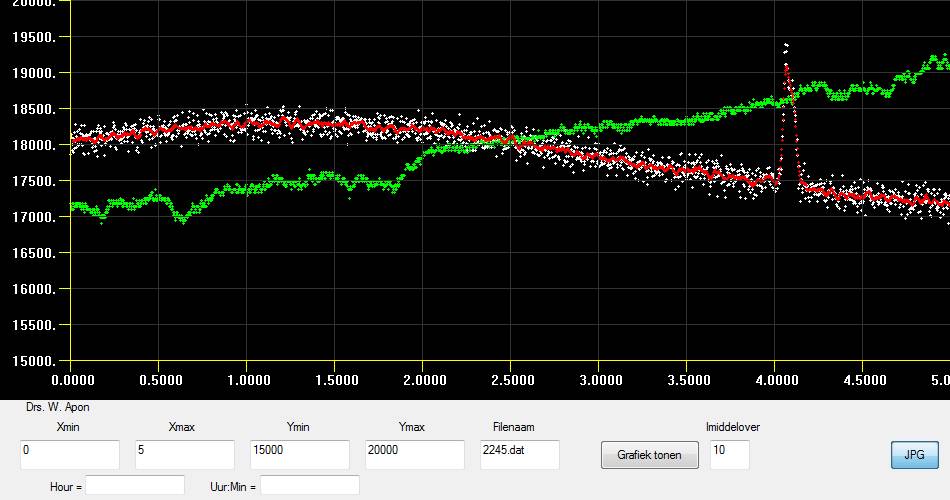
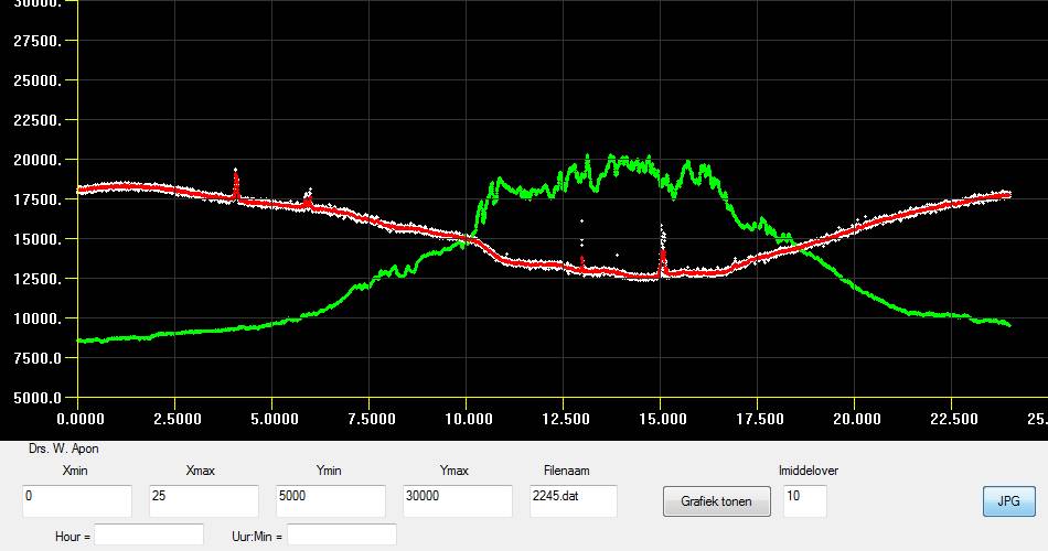
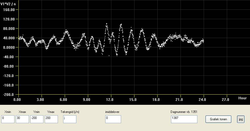
5 days drift scan of the sun.
first day is white, second is red, then green, blue and yellow.
The maximimun shifts every day 1 minute.
the graphs show only the running mean of 10 values.
At the left side of the left slope you see a side lobe of the
antenna system.
Horizontal scale is time in hours UTC and vertical a sort of voltage.
24-10-2012
I plan to measure the sun for about 10 days and see what happens.
I do not change anything... just continuous measuring.
At this moment i already have 4 very nice pictures of the sun passing.
In the mean time i am thinking about my new experiment.
The phasing interferometry with 4 antennas and 4 ssb receivers
at 150 MHz.
21-10-2012
Yes, i measured the sun!!!
Now i can get an idea about the openings angle of the system
and the sensitivity. ( not very sensitive!!)
The openings angle is something like 2 degrees.
20-10-2012
Ohhh still nothing to see in the graphs.
So i did change the orientation of the disk to the sun.
This was an easy job, because the sun was shining.
I only had to turn the disk in a way that the shadow of the
LNB was at the centre of the disk.
7-10-2012
I start to do 2 weeks of measuring and changing nothing to get
a feeling of what i am measuring.
The disk is still pointing to the point where Cassiopeia-A will pass.
6-10-2012
Ohhhh nothing to see... i do see only a changing in signalstrenght
by day and night. I think this will be caused by temperature.
3-10-2012
The system is ready.
When i connect a spectrum analyser to the LNB i can see some
noise caused by satellites. So the system is okay!
So today starting measuring at 12 GHz with the disk orientated at a point where
Cassiopeia-A will pass. ( Azimuth = 40 degrees and Elevation = 40 degrees
Pass at 15:15 UTC)
1-10-2012
After a break of a few month i decided to do a quick and dirty experiment
with a 12 GHz rig.
A few years ago somebody gave me an old 1.5 m disk.
Now it was nice to do an experiment with it.
(Just thinking about something else than phasing interferometry for
a few days)
I found a LNB and started setting up the installation.
In house a had all the needed apparatatus and most of the software.
Phase Interferometry

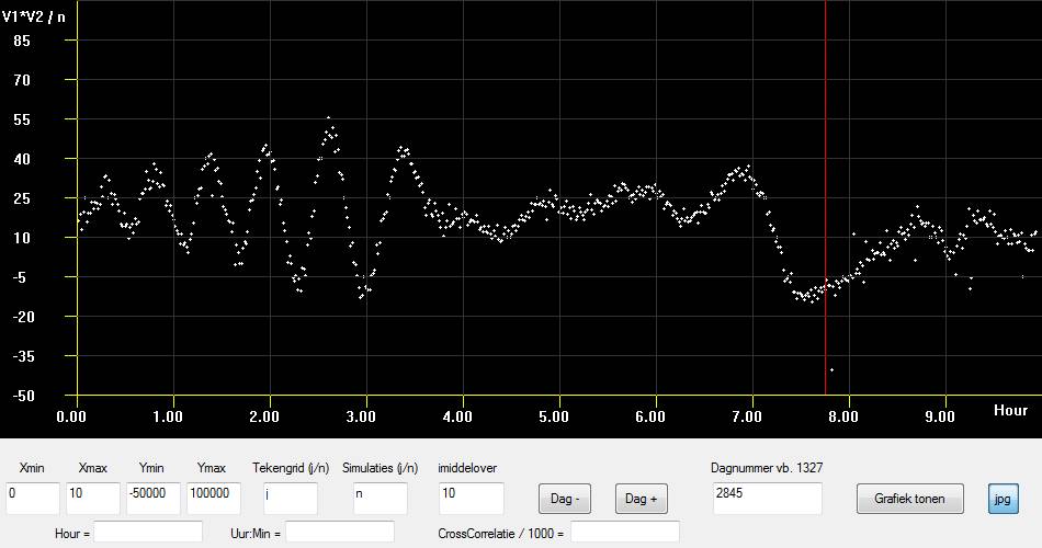
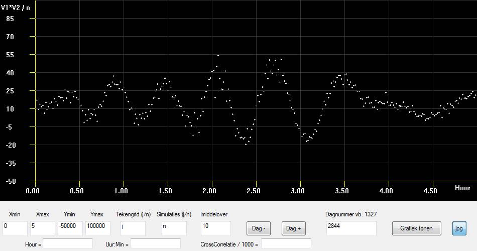
Above the 19 measurements plotted at different heights in
the graph. It looks good.....
(Only the walking mean of 20 minutes is plotted)

Above the same 19 measurements plotted at the measured y-axis
position.
What you see is the socalled daily variation.....
Again only the walking mean of 20 minutes is plotted.
So i concluded that the daily variation of any measurement
gives a variation of 20 percent of the amplitude.
(the bandwith of all the curves along the y-axis)
So any crosscorrelation value has a fault range of 20 percent!
I think The 2D-FFT algoritme that makes the maps of the
radio sky can handle this..... ( i hope)
1-5-2012
All sceduled measurements are done.
In night time the measurements are usable, in day time not!
Now i am measuring for some 20 days with the same base line to
get a good insight in the so called "daily variation"
I will here publish all this 20 measurements when they are done.
In the mean time i start calculating a lot of maps of the sky.
5-3-2012
The new measurements give splended results.
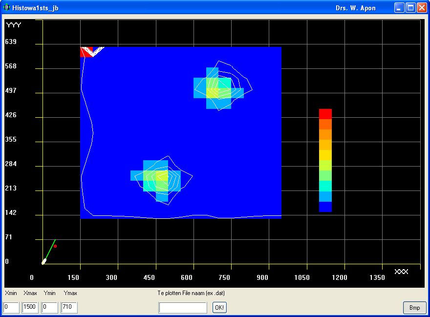
Below you see a map of the sky with only 25 measurements.
13 new ones ( the left part with the shortest baselines) and
12 old ones ( of a year ago ) ( the right colums)
At night times the measurements are perfect, but during the daytime they
are hopeless.....
The upper circle is Cassiopeia-A
The middel circle is Cygnus-A
The lower circle is the milkyway.
16-2-2012
After a long time of trouble, i can start measuring again.
I have to measure the short distances again ( the last 90 measurements)
17-12-2011
The antenna amplifier is repaired.
the first fringes are seen now.
First i am going to put the astrorover at known locations to check
the fringe picture and then i can calibrate the time problem
with the latest 90 measurements...
7-12-2011
HOUSTON WE HAVE A PROBLEM
------------------------------------------------------
One antenna amplifier broke down. The transistor is blown up.
And, the computer which did measure the last 90 days, had probably a wrong running clock.
It was running at dutch winter time, but i am not sure.
So i have to do a few days measuring to check the time calibration.
But i can not measure now.
First repair the amplifier. I have to find the good transistor and than replace it.
But i made the amplifier so small and did use so much copper shielding that i have
to dismantle the complete box.....It is a bloody job.
28-11-2011
A new -9 volt dc-isolated power supply cube arrived.
Now the receivers are working nicely.
17-11-2011
The receivers stopped working. One of the power supplies stopped... ( the receiver
uses 4 power supplies... ( 3 Volt, 5 Volt, 12 Volt and a -9 Volt)
The -9 Volt one stopped.
15-11-2011
I had to stop measuring because of "conditions" on the HF-bands.
At day time i do receive too much earthbound disturbances.
10-11-2011
Most of the interferometry measurements are corrected now.
(Automatic data collection from the measurements to make maps of the sky
can not use faulty data)
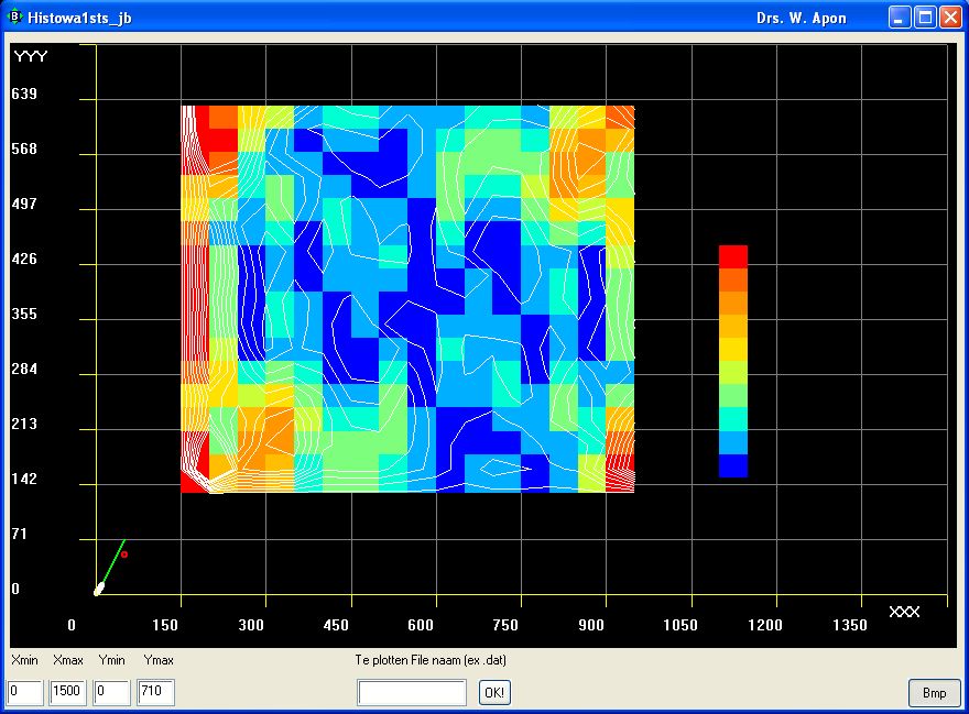
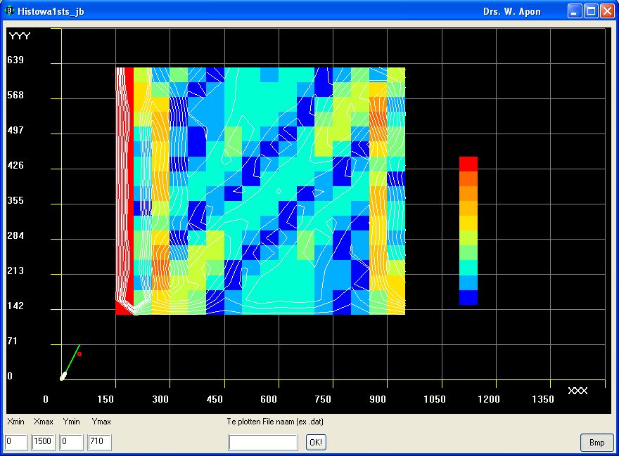
Below you see a raw data measurement and the corrected version.
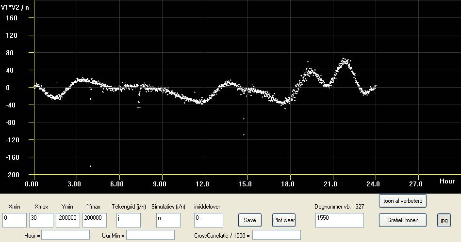
Above a raw data graph
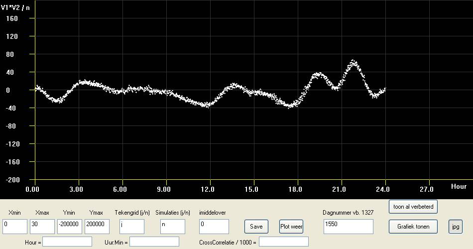
Above the same graph but now corrected.
19-9-2011
In 200 days i collected 1 TByte of raw interferometry data.
Next weeks i have to correct faulty data
For that i am writing a grafical correction program.
26-8-2011
Still measuring with short baselines, but daily thunderstorms disturb the results.
17-4-2011
My new Pure Basic 2D-FFT program is a fabulous tool !
Because i can not do now real star measurements i decided to do some stand-alone experiments.
I took an old computer with an unknown soundcart and installed it in the caravan.
I put a noise-transmitter at 250 m. from my antenna field and measured a lot of positions with
the astrorover.
I did 42 measurements and calculated maps with a different amount of measurements.
With only 4 measurement you get allready some sort of a map.
with 9 measurements the map is some better.
with 16 measuremts it is allready a real map.
with 25 measurements the map is better.
with 36 measurements the map is still better.
with all 42 measurements the map is the best of all and the direction of the found source is
exactly the azimuth of the noise transmitter.
See the maps below
So i am sure my method of measuring is good!
15-4-2011
The measuring computer crashed..... The hard disk crashed.
So, for the time beeing i can not measure anymore.
14-4-2011
I had a good look at my new 2d-fft program ( now in Pure Basic) and saw that it gave a nice map of the
sky. Only north , south east and west where at the wrong position, but flipping each quadrant
solves that problem.
I don't know why, but the old Quick Basic program did not gave a readable map....
So, while not knowing why, i am happy with the new results.
Now i could do the quadrant-flipping and did some cosmetics on it to produce nice maps.
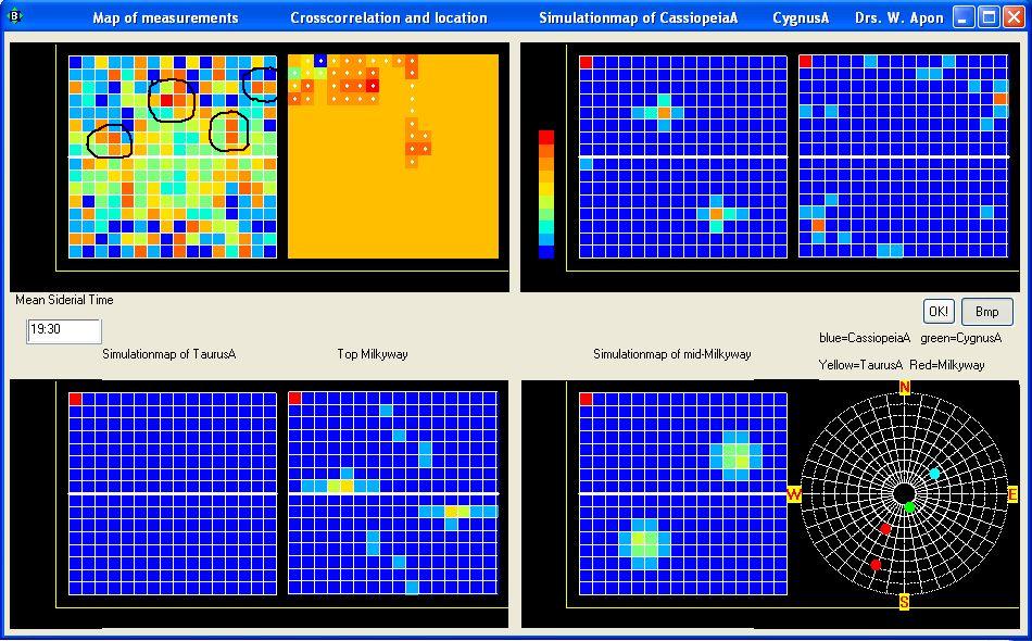
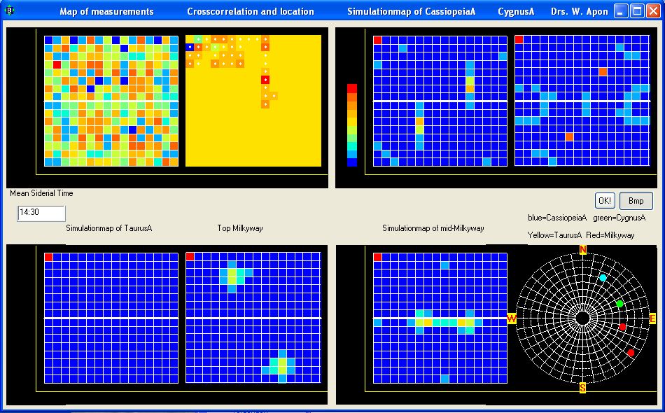
Below you see a map calculated and plotted with the new Pure Basic programs.
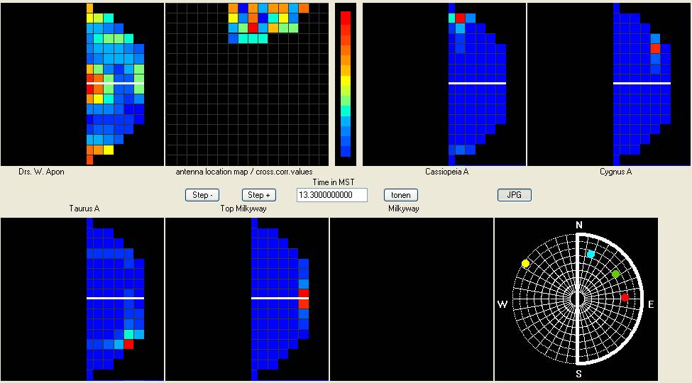
You see the measured map top-left.
More to the right you see the positions of the astro-rover ( second antenna) and the crosscorrelation
values of that positions. Norht is above and the first antenna is top-left.
Further you see the simulated maps of CassiopeiaA, CygnusA, TaurusA, and 2 of the milkyway.
Bottom-right is a normal star-map of the radiosky.
Blue dot is CassiopeiaA, green is CygnusA, yellow is TaurusA and red is the milkyway.
For all maps: the north is above, the south is bottom and east is at the right side.
The elevation is at circles whith 90 degrees at the middel of the maps.
Because the left part of the map is symmetrical i did not draw it.
So TaurusA has an azimuth of 315 degrees, but it will be measured and plotted at 135 degrees.
You see most of the simulated radio-sources in the measured map at about the same position as
in the simulatied maps and in the map of the sky bottom-right. TaurusA is to week to see.
1-4-2011
I am halfway my measuring scedule and the results are great.
Below are 2 plots of the results.
I did now use new programmed Pure Basic compiled software.
The program which does the 2D-FFT calculations and the plotting has about 4000 basic code lines.....
The calculation of the crosscorrelation together with the temperature compensation is an
other program. This program uses 15 minutes of calculating for 1 day of measurinig. (!)
(Realise one day of measuring gives 4.5 GByte of data)
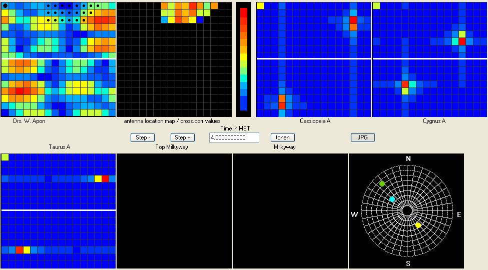 Upper left graph is the result of the 2d-fft calculation of the measurements, together with the locations
of astro-rover ( black dots). More to the right is a location map of the astrorover ( second antenna).
The color represents the relative value of the crosscorrelation at this position.
Below right is the normal plot of the known radio sources at the sky.
Blue is CassiopeiaA, green is CygnusA and yellow is TaurusA. Red are 2 parts of the milkyway.
All other graphs are simulations of this sources in the same way i calculated the map upper left.
31-3-2011
I am now halfway my mapping scedule.
I transfered all my Quick Basic and Just Basic programs to Pure Basic.
I learned a method to corrigate for temperature variances in the antenna amplifiers.
So the day to day temperature problems are solved.
The first mapping results are growing.
In a few days i will publish a few maps here.
31-1-2011
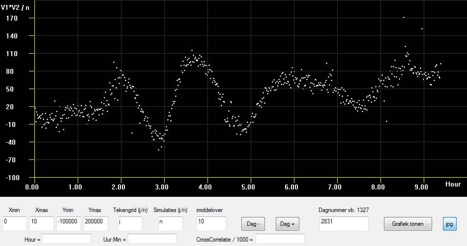
Below you see one of my new measurements with the soundcard and 36 seconds of measuring per minute.
Base = 54.6 m. West-East freq = 30.984 MHz
22-1-2011
I am using now a soundcard as digitiser.
TheFigure below shows the difference
between my old measurements and the new ones.
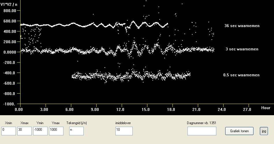
All my measurements until now are done like the lowest curve.. ( I digitised
every minute for 0.5 sec)
The middle curve is digitised with the soundcard for 3 seconds per measurement.
The upper curve is done with the soundcard for 36 seconds per measurement.
So, this will improve my maps!!
I will start now with a new mapping scedule.
12-1-2011
Last months i was busy with a new compiler, to calculate and make the graphs.
It is the Pure Basic compiler.
A very fast, modern compiler, which is windows orientated. It works also under Linux.
This compiler can handle a computer soundcard. So this gives new challenges!
I made a setup to measure every minute for 3 seconds.. i get then 66000 samples per antenna.
I costed me 3 weeks to translate the quick basic programs to this new compiler.
In the mean time measuring everyday.
I made the grid smaller... grid distance is now 4 meter. (was 8 meter).
I had no time to make maps....
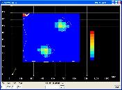
1-11-2010
You should say: you see 4 sources.....
29-10-2010
Still measuring every day
I also made some extra software, to get a better overview of the measurements.
Below you see 37 days of measuring. Every line is one day measuring.
The time x-as is in MST. (not UTC)

This 37 measurements give at 14:30 MST the map below.
I made some nice examen programs
First results are found
(6 june 2010) The last months i was busy creating and adjusting the new
rig to do the phase-interferometry.
above, both receiver channels got the same 1000 Hz signal.
18-10-2008
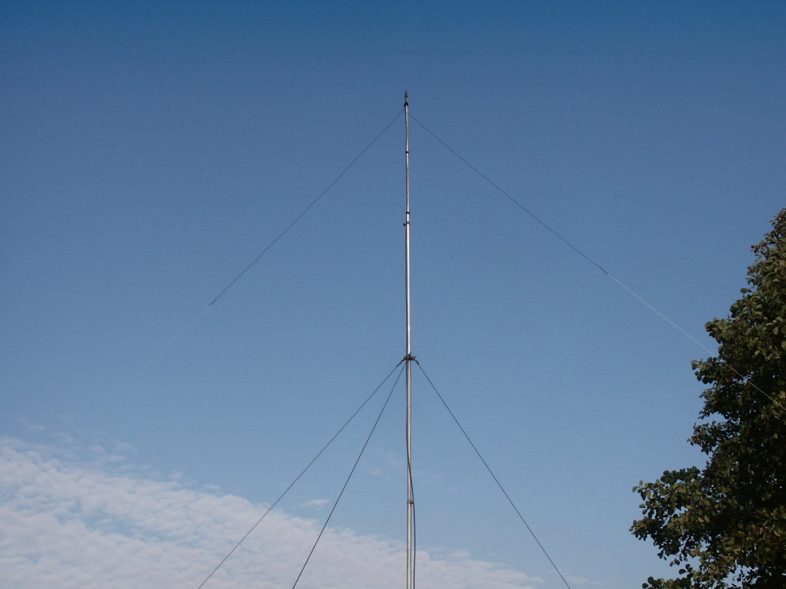
De Inverted-V dipole van dichtbij. Hij is bemeten voor 25.6 MHz.
Ik hoor de hele middag op 25.6 MHz al de branding-ruis-geluiden die
van Jupiter komen.
Helaas bleken deze mooie geluiden uit de ontvanger zelf te komen, en dus niet van jupiter.
27-10-2008 Ik ben bezig geweest om een tweede AVR-computer te bouwen. Deze computer kan
elke 2 seconden het azimuth ( en de elevatie ) van een ster berekenen. (Zie het programma
VINDSTER.BAS van de software pagina.)
Tevens draait hij de antenne naar het berekende azimuth.
Als test ga ik een paar dagen de antenne op de zon gericht houden,
terwijl de oude AVR-computer elke 8 seconden een ruis-sterkte meting doet.
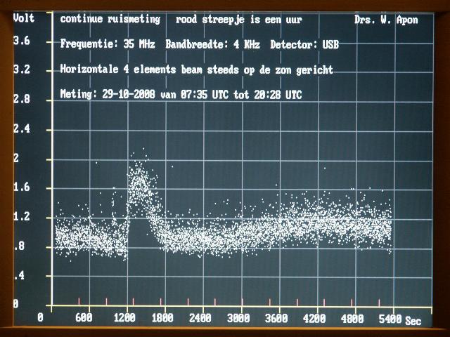
29-10-2008
Kassa! een zonneuitbarsting gemeten.
Zonneuitbarsting van de zon gemeten op 29-10-2008
Hij begint ongeveer bij seconde 1200 en eindigt bij seconde 1800
Dit is de klassieke vorm van een uitbarsting: snelle toename en langzame afname van de ruis.
The figure right below is a calculated map of the sky here in Delfzijl at the same time
as my measeured map.
It is good to know that the milkyway is a broad line of radiosources from what i call "top milkyway"
over the "mid milkyway" to outside of this picture.
9-10-2010
Probably there is nothing wrong in my software, so i think i have to live with the ambiguous
character of the results and simulations.
So i decided to do it the other way around: ( not very scientific...... )
First calculate a map of my measurements, than make simulationmaps of the brithtest radiosources and
then try to find the simulated sources in the map.
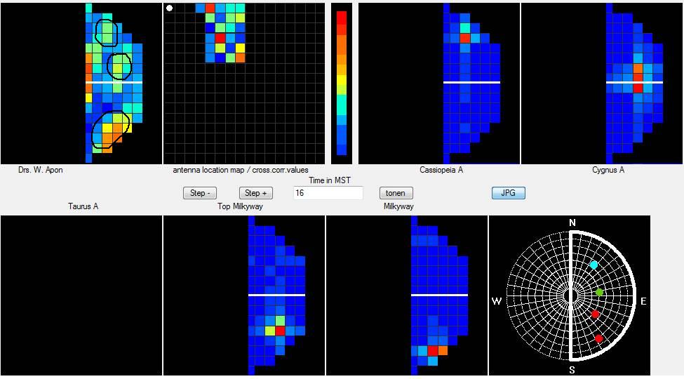
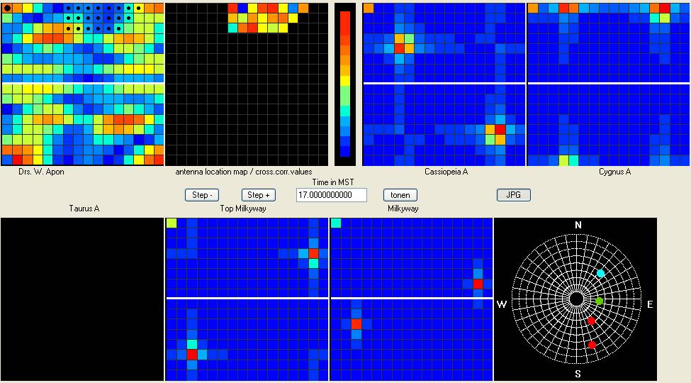
Therefore i made some overview software:
In one picture i can see the map of my measurements, the location of the used antenna positions,
the simulated maps of CassiopeiaA, CygnusA and the milkyway (or TaurusA)
Because of the way of sampling, i can make a picture for every minute.
At some moments i can find the simulated sources in the measured map.
At other moments it is completely rubish....
In the mean time i take every day an other location for the antenne and continue the measuring.
25-9-2010
There is something terribly wrong with the maps i can make now.
When i simulate posititons for CassiopeiaA for all 24 hours a day, i see that it comes a few times at the
the same location on the map.
That is rather ambiguous... so my maps do not tell where the source is!!!!
SO, WHAT TO DO NOW???
20-9-2010
I made some nice programs:
A 2D-FFT program, A mapping program and a 2D-Simulation program
My mapping sequence will follow a rectangular 16 by 16 grid with nodes every 8 meter.
Every measurement will will take one day of measuring.
This 256 measurements ( 256 days of measuring.....) will give me a map of the sky.(i hope)
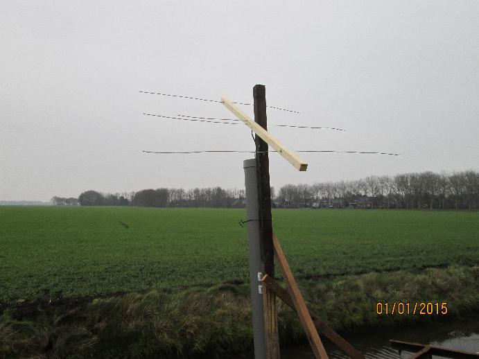
At node (0,0) stands one inverted V antenna.
The other inverted v antenna ( on the astro-rover) will stand every day at an other location,
following the 16 * 16 grid.
So i get every day a graph like i showed earlyer.
To be sure that the whole thing will work, i made a simulation program which calculates the
crosscorrelation value of every antenna position in the grid on a certain time. Let us say at 01:00 Hours MST.
Then i made a mapping program which can show all values at the right position within the grid.
It is a program which shows 16 * 16 coloured pixels. Every pixel is one antenna position.
Because the pixels give a coarse picture, i made a contouring program as well.
This program shows contourlines within the pixelmap.
Now slopes in values are clearly visible.
To be able to make a map i developped a 2d_FFT program.
I am not sure... but they say: it will give a map.....
When i did experiment with this 2d_FFT program it was clear that it delivers a map indeed.
So i can now make a map of my simulated data, and maybe of my real measurered data.
A map of the simulated crosscorrelations at 03:00 hours Mean Sideral Time.
The map has 2 identical parts. The upper and the lower part. This parts are mirrored.
I don't know why... but i can live with it.
The yellow dot is the position of CassiopeieA at 03:00 hours MST.
To control all program's i made a map for every hour. This proved my program's are correct.
01:00 MST
02:00 MST
03:00 MST
04:00 MST
05:00 MST
06:00 MST
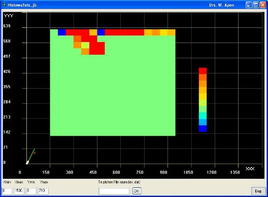
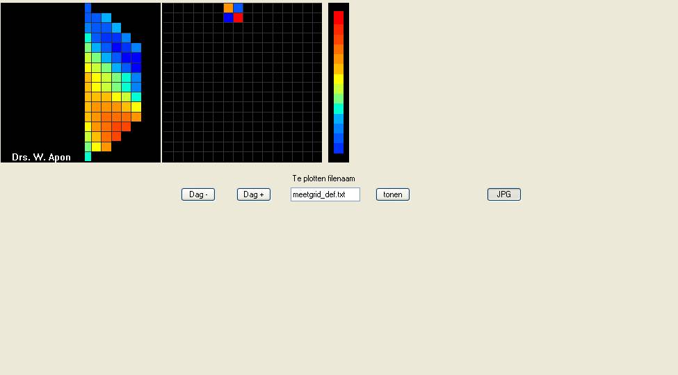
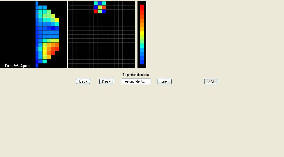
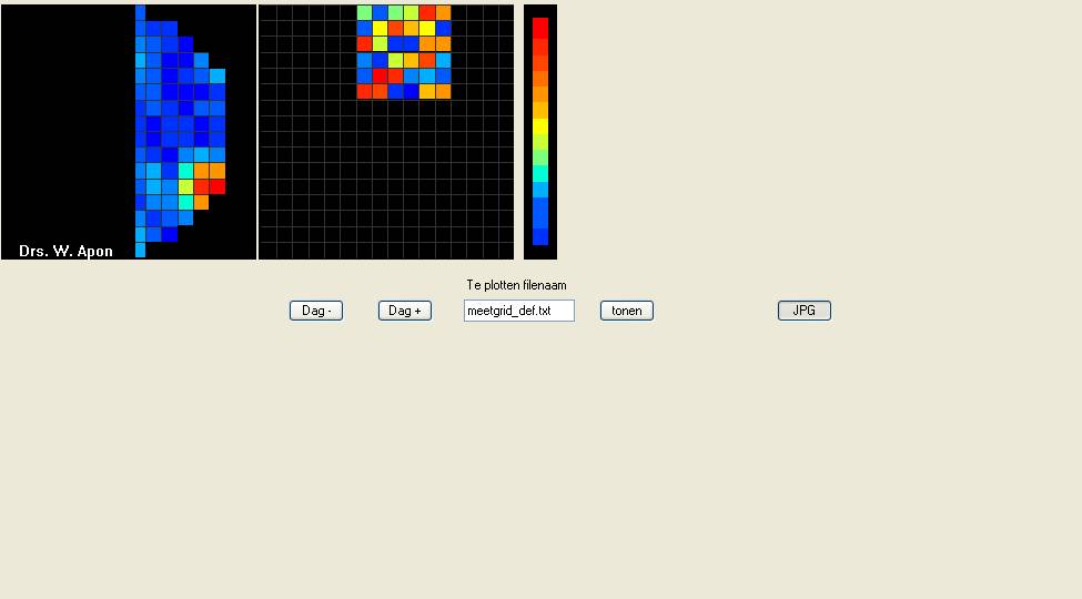
Above:
For every measurement, i made until today, you see one square at the top of this graph.
So you see 25 measurements. The color is the value of the crosscorrelation value at
0.4 Hour MST. The North is pointing to the top of the map.
Above you see the map i made with this 25 measurements....
In the upper-right corner you see CassiopeiaA..... ( i hope....)
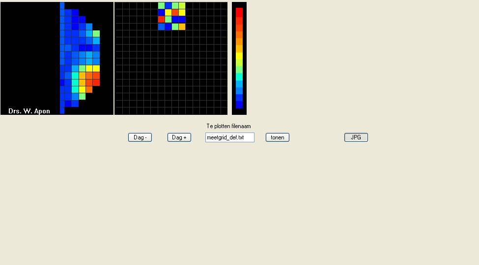
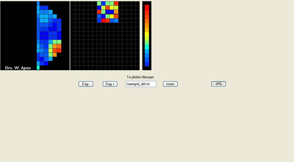
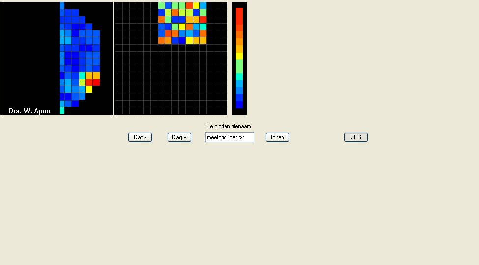
Above you see the map i calulated from the simulated crosscorrelation values of the same 25 grid nodes.
In the upper-right corner you see CassiopeiaA.
30 august 2010
Before i can start my mapping program, i needed a method to change one antenna to lots of places
without too much difficulties.
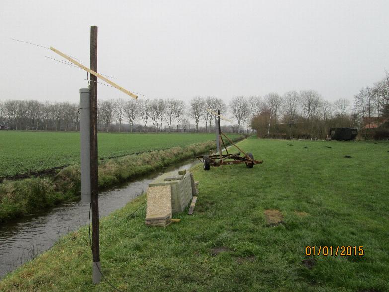
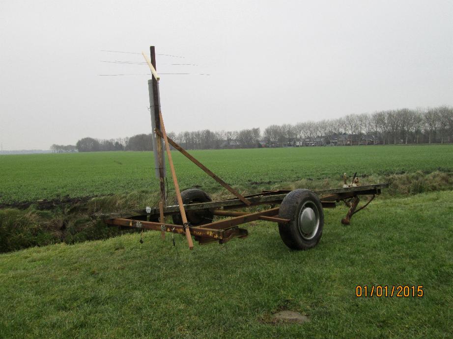
Therefore i made a small vehicle with an antenna on top of it, and i called it: The AstroRover.

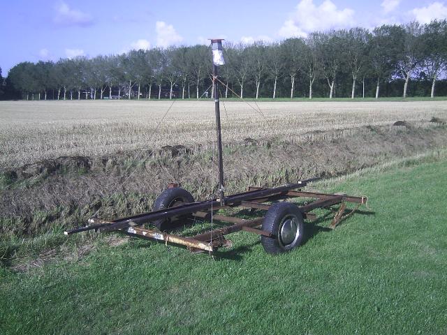
The AstroRover.....
I put the antenne on an old metal frame of a caravan, and so i
can move the antenna to any place i want in a few seconds.
The wind can not blow it away because it is quit heavy.
Now i can start my mapping program. I will put the antenna every day at an other place,
following a rectangular grid.
First grid will be 4 by 4 positions. ( So 16 days of measuring)
In the mean time i can create the software programs to make a map of the sky.
I also try to get, compile, and use the Miriad software program.
Miriad is an radio interferometry data reduction package for users of the
Australia Telescope Compact Array (ATCA)
It is a free program which is running on Linux computers.
So i took an old PC and put Ubuntu (Linux) on it, and tried to compile the Miriad progam...
.... a hell of a job......
But maybe i will succeed.....
BR>
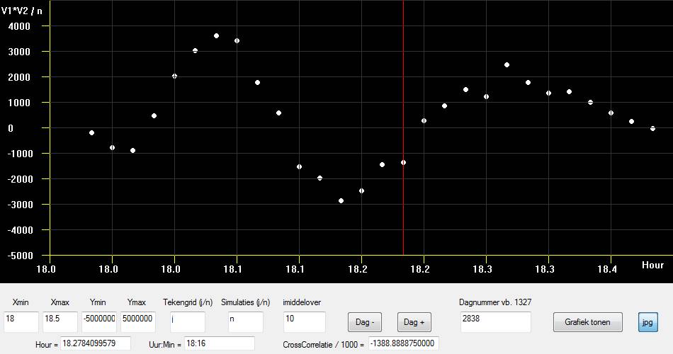
16-July-2010 This program shows all the information of one day measuring.
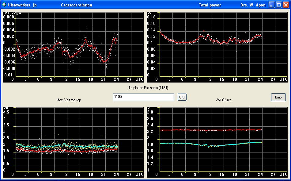
Above results of the 15-july-2010 day measuring. Base = 8.54 m. Freq = 31.0 MHz
Top left is the cross correlation of the two receiver signals.
Top right is the total power of the same signals
Base Left is the maximum top-top voltage of both signals.
One receiver produces some more signal than the other.
Base right is the offset voltage of both signals which are being digitised
by the digitiser. Because this digitiser only can digitise voltages between zero
and 5 volt the receivers produces this offset voltage.
to calculate a crosscorrelation, you must subtract this voltage from the measured
voltages to get a nice graph.
In fact this offset voltage for this graph is calculated as the mean voltage of all
8192 ad-samples for one measurent of 0.5 sec.
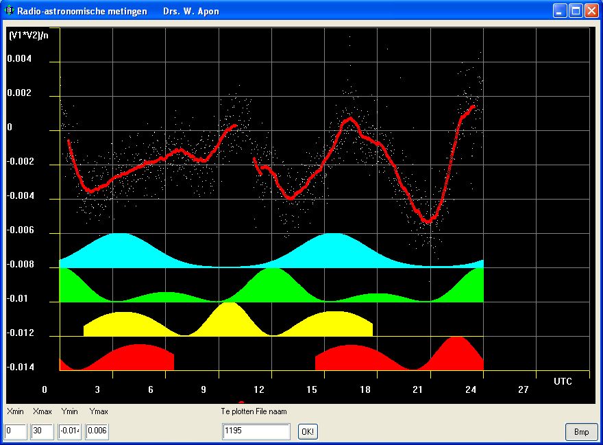
Above the cross correlation of the same measurement in more detail and with a
simulation of 4 possible sources.
Blue = CassiopeiaA
Green = CygnusA
Yellow = TaurusA
Red = Top Milkyway
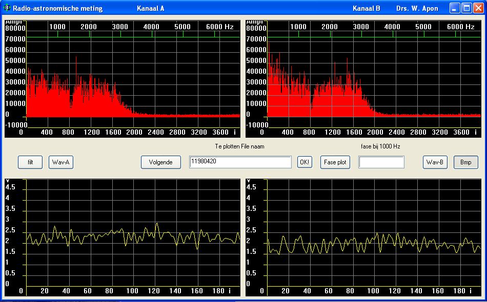
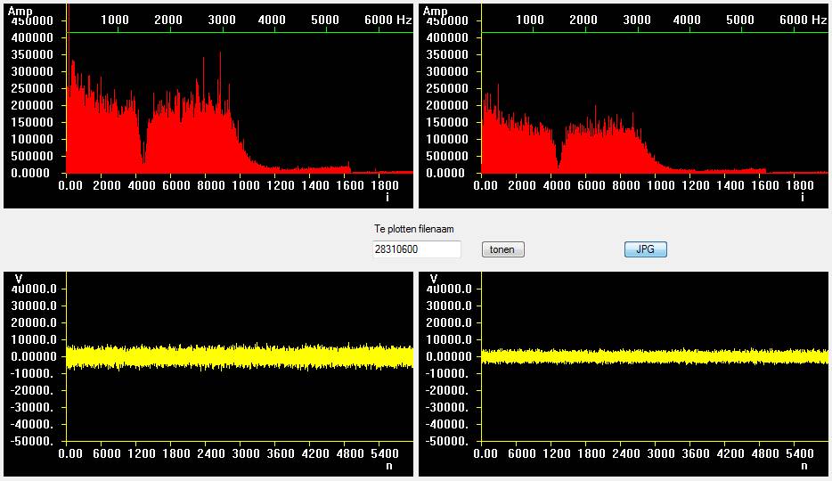
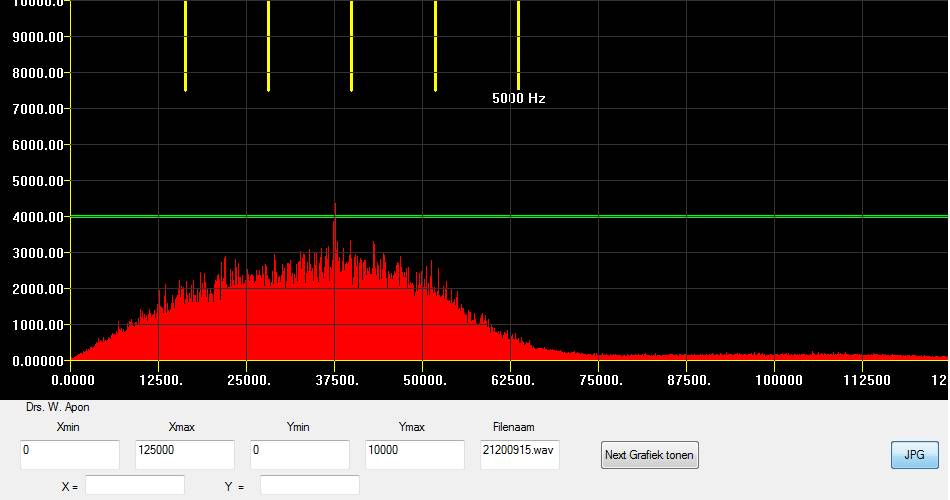
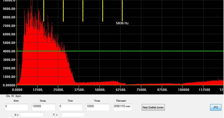
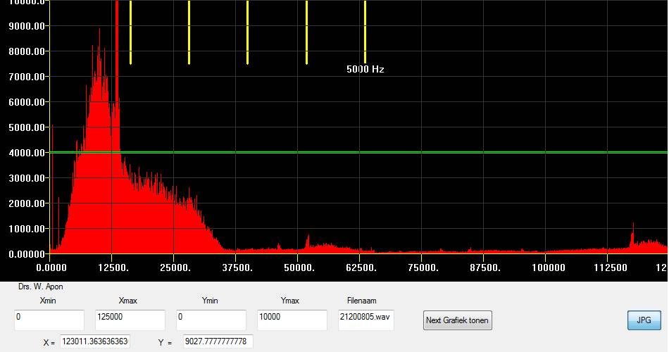
Above is a picture of the program which i use to examen 0.5 second of measuring.
i can see the frequency spectrum of both receivers
when i push the WAV button, i hear the sound of this 0.5 seconds.
The first fringes are seen.
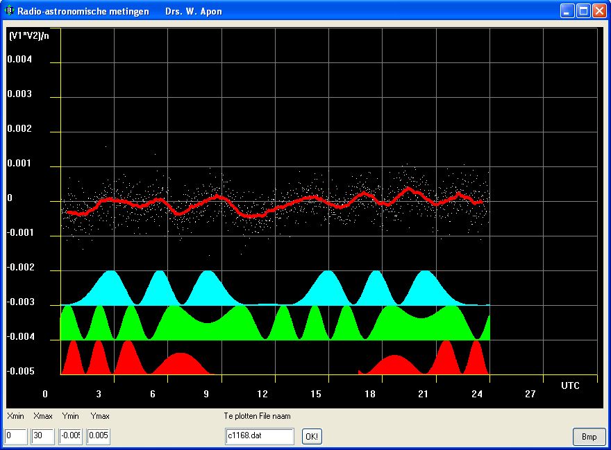
The first quick and dirty results, a cross-correlation of the two receiver signals.
below the 3 simulations:
upper : CassiopeiaA
middle: CygnusA
below : Top Milkyway
The curve is measuring result of 18 june 2010
The software is almost ready; the digitiser is ready and works perfect.
The two coherent receivers will be ready in a few days.
The software i wrote in Just Basic, a free basic compiler with a windows alike look.
Just now a few examples of it.
the fase interferometry telescope uses 2 antennas, 2 coherent receivers and one digitiser.
The digitiser samples both receiver signals.
So the first sample is from receiver A and the second sample is from receiver B,
the next sample is again from receiver A and so on.....
The software makes for every channel one file and does a Fast Fourier Transformation on it.
The results gives the next graphs...
At least the software calculates the phasedifference at 1000 Hz between both signals.
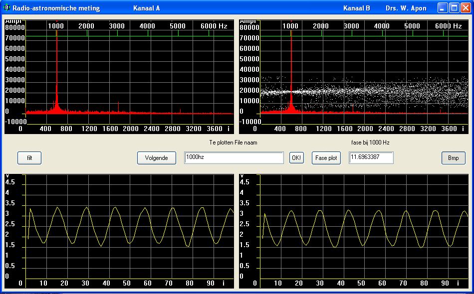
The left upper and bottom graphs shows channel 1
the right upper and bottom graphs shows channel 2
the upper graphs shows the frequency spectra
the lower graphs shows the received signal ( the first 100 samples)
The upper right graph shows the phase difference between the two signals as white dots.
The phase diference at 1000 Hz is shown in a small text box in the center
This phase dots are scaled to fit into the graph.
When a phase dot is on the horizontal line of 20 000 the phase is zero.
You see that the phase difference increased with increasing frequency.
I think i have to filter the receiving signals...... ( is that so?)
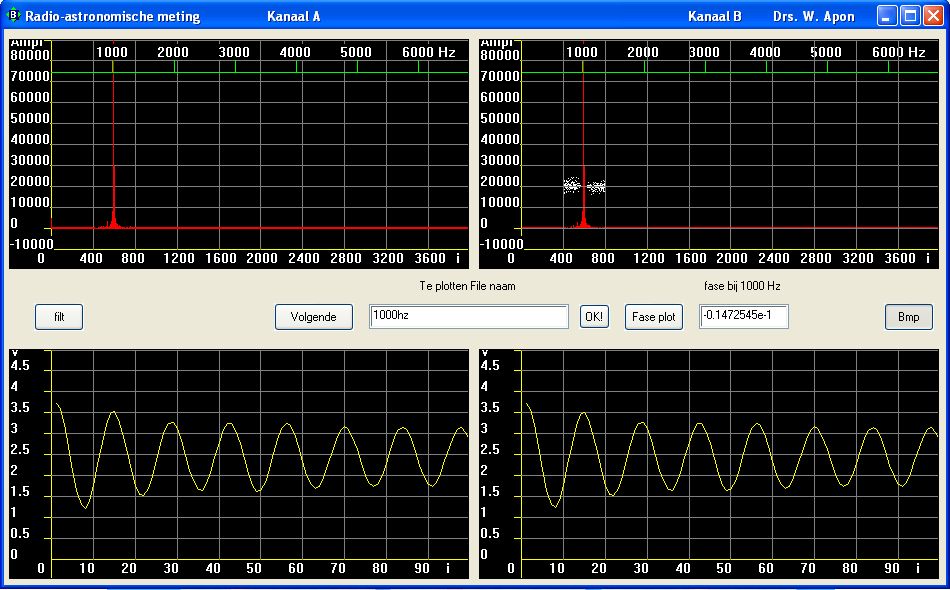
the graph above shows the result of a filtering with a band-pass filter.
It filters the signal between 400 and 800 on the x-as. That is about 700 to 1300 Hz.
as a result the phase difference is changed to about zero...
So here is a problem, because the phase did not change.......
I do have a big problem...
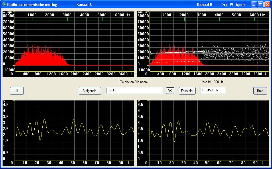
Above you see what happens when i couple the lf-output of one receiver to the digitiser.
The receiver has a bandwith of about 3000 Hz.
The phasedifference between both signals is increasing with frequency.
This is caused by the way of sampling... For this the phase values must be
corrected. The graph shows clearly this effect!
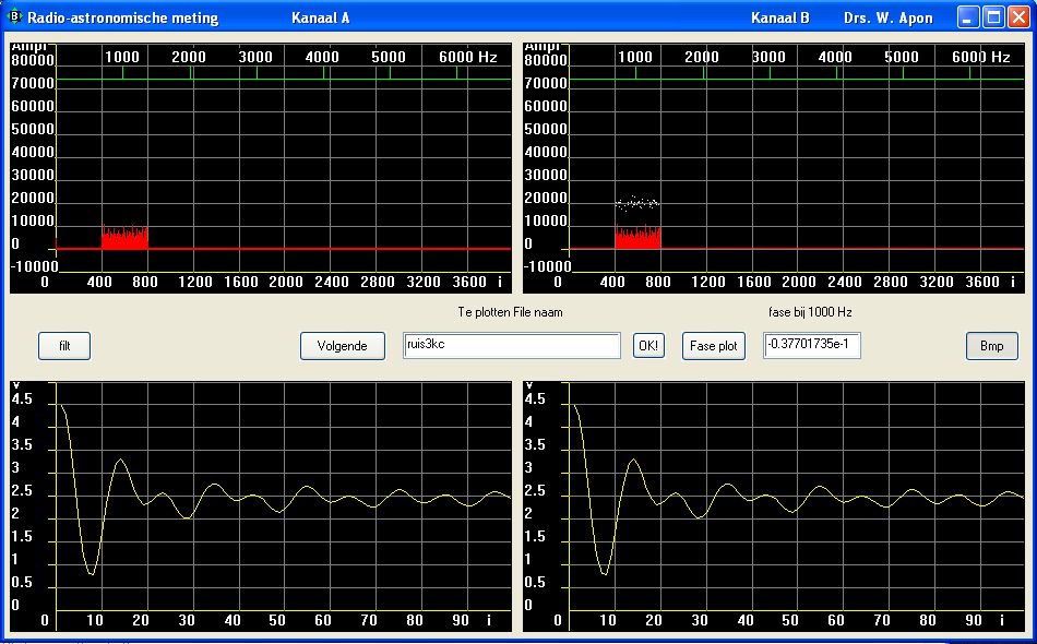
Above you see again the filtering problem.
The signal is now again filtered between 400 and 800.
The phase is for the whole bandpass about zer0.....
I do not know what to do with this problem.....
Klaar voor de ontvangst van de Jupiterstorm van vanavond. Even een inverted-V dipole
op 8 m. hoogte geplaatst. Een tweede AR3000A ontvanger staat in de caravan buiten beeld.
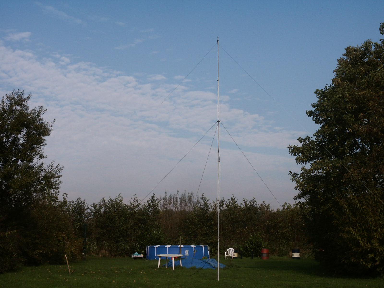
Op 35 MHz hoor ik ze niet, ook al richt ik de 4 elements beam op Jupiter.
5-11-2008
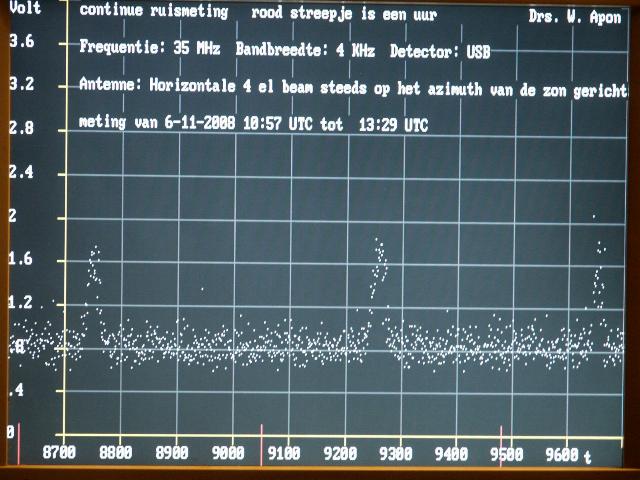
De laatste dagen steeds continue metingen uitgevoerd. De antenne volgt constant het
azimuth van de zon. Ook al zit hij onder de horizon.
Het zijn metingen waarin niet zo veel gebeurt.
alleen op 6-11-2008 zie ik weer een aantal spykes.
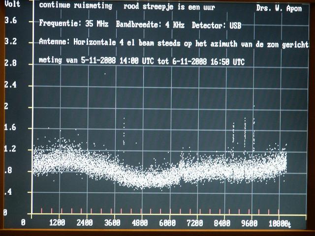
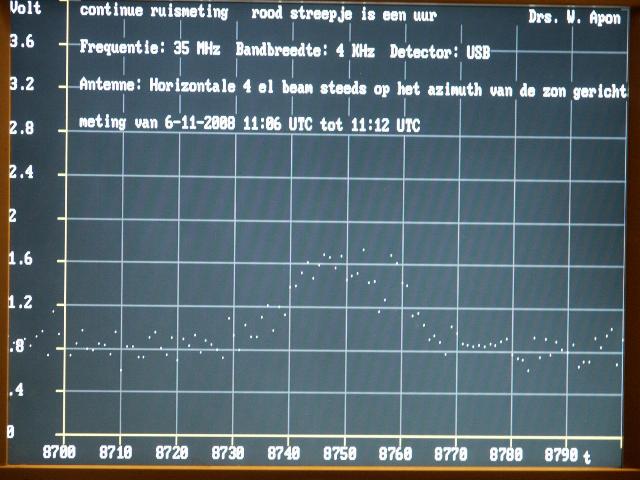
De 3 spykes rechts op bovenstaande foto's uitvergroot.
De meest linkse spyke van bovenstaande foto verder uitvergroot
van de spyke aan.